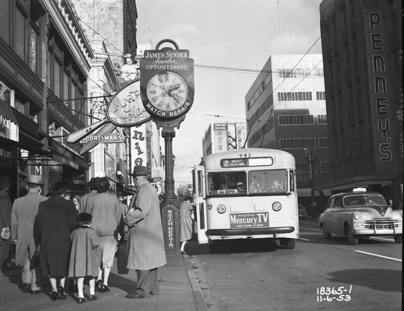
“City bus, 1953” by Seattle Municipal Archives is licensed under CC BY 2.0.
The contention that the average commute duration has remained constant over time, and is independent of cultural differences and the built environment, underlies Marchetti’s constant. Technological changes might determine how far one can go, but the time allotted remains the same. That allotment is thought to be an hour total, or 30 minutes each way. I came across Marchetti’s constant early in my exploration of transit planning, and my analyses typically use a time budget of 30 minutes. That being said, I never made an explicit decision that I would use that time budget because it’s Marchetti’s constant. That 30 minutes seemed like a reasonable amount is probably influenced by having encountered it, though.
In spite of that choice, I simply don’t like the idea of assessing the quality of transit using a parameter justified by Marchetti’s constant. That a preferred amount of commuting time is built into human nature seems preposterous. While it’s interesting that this average value shows a persistence over circumstance and time, is there any merit to the average value itself? It feels like the sort of average that folds a diversity of individual preferences into a single, flawed description of a human stripped of agency. There are plenty of people who will tolerate longer commutes, and plenty who would balk at devoting an hour per day to it, and plenty whose tolerance varies depending on the current priorities in their lives. There are trips that people need and want to take that are not part of commutes. How long should be considered tolerable for those? Contemplating what people collectively “prefer”, “are like”, or “will do” seems to inform decision making in the transit planning field, but individuals, not populations, make the choice to board a transit vehicle.
Making statements about transit quality using an access measurement for a single duration is something I have done regularly, but generally should be regarded as insufficient. My first post outlined some objections I have with transit consultant Jarrett Walker’s particular applications of access measurement. I critiqued a 30 minute time budget as producing an artificial binary between “too long” and “short enough”. I deemed it only useful for reducing computational outlay, and that it should be regarded as a limitation, not a feature, of the measurement. Positive changes to transit networks should allow more journeys to be completed for every possible time budget. A good measurement should be able to verify whether this is true.
Looking at the access for a single duration would be sufficient only if it provides pertinent information about all other durations. If a change to the network is made, and 30 minute access improves, can the access improvement for a 45 minute time budget be estimated? Perhaps cities have transit networks that are optimized for different lengths of trips. Will looking at the 30 minute access for two cities give a false impression of which city has better transit overall?
To explore these questions, I performed access analyses with varied time budgets in Seattle and Milwaukee. In Seattle, I considered both the current transit network and the proposed restructure that I previously created. For Milwaukee, I reused the same map and schedules from my previous analysis of multiple cities. The durations that I considered were every multiple of five between five and 60 minutes, and every multiple of 10 between 60 and 120 minutes.
Technical Interlude
“KCM 2398 with exposed engine” by SounderBruce is licensed under CC BY-SA 2.0.
Before examining the results, I want to discuss how access computation works with multiple time budgets. There are two phases. The first phase is pathfinding. This involves discovering the shortest-time path of walking and transit trips between all sectors, for each minute of the day. The second phase is aggregation, which is transforming the pathfinding results into useful data. The simplest version of this counts the number of times each sector has been reached, which is used to create the access maps. There are also aggregations to calculate how often routes appear in the results or the sequences of routes that are most common.
When considering multiple time budgets, it is only necessary to perform pathfinding once. In general, the duration is used to end pathfinding early; it’s fruitless to continue trying to find a path between two sectors once over budget. Pathfinding only needs to be run for the longest duration. Once the paths are computed, their duration is known; the aggregation step for each of the shorter durations considers only the paths shorter than the duration in question. This means that there is a computational time cost to adding new durations, but it is not as severe as completely re-running the full analysis for each added time. I considered analyzing durations of every minute between one and 120, but settled on 18 of them after considering the nontrivial aggregation cost of the former.
Seattle: Existing and Restructured
For the 18 durations, I wanted to compare Seattle’s existing transit network and my proposed restructuring of it. In specific, I sought to understand whether the restructured network is always better, or if the existing network outperforms it with time budgets other than 30 minutes. I plotted the access ratio for both networks, for each time budget. Both followed a similar pattern, resembling a logistic curve. I didn’t anticipate this, but it makes sense in retrospect. A logistic curve grows exponentially before converging towards a maximum value. The proportion of the total sectors that can be reached will never be greater than one. I used the Nelder-Mead method to estimate the unknown parameters k and x₀ in the logistic function, and added the curves to the plot.
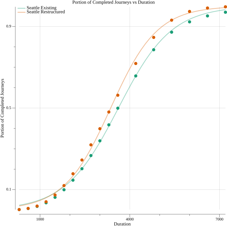
Seattle existing parameters: k=0.001124 x₀=3619, Seattle restructured parameters: k=0.001277 x₀=3360
At first glance, the curves do not appear to be terrible fits, but they overestimate the access for short durations. The following table explores the estimation error for the current service in Seattle. The equivalent data for the restructured network follow a similar trend.
| Duration (Minutes) | Expected | Actual | Error | % Error |
|---|---|---|---|---|
| 5 | 0.023 |
0.002 |
0.021 |
1025.83% |
| 10 | 0.032 |
0.007 |
0.025 |
340.89% |
| 15 | 0.045 |
0.018 |
0.027 |
153.91% |
| 20 | 0.062 |
0.035 |
0.027 |
75.16% |
| 25 | 0.084 |
0.062 |
0.022 |
35.90% |
| 30 | 0.114 |
0.099 |
0.015 |
15.35% |
| 35 | 0.153 |
0.146 |
0.007 |
4.84% |
| 40 | 0.202 |
0.202 |
0.000 |
0.00% |
| 45 | 0.262 |
0.267 |
0.005 |
1.75% |
| 50 | 0.333 |
0.339 |
0.007 |
1.98% |
| 55 | 0.411 |
0.418 |
0.007 |
1.56% |
| 60 | 0.495 |
0.499 |
0.005 |
0.96% |
| 70 | 0.658 |
0.658 |
0.000 |
0.00% |
| 80 | 0.790 |
0.786 |
0.004 |
0.56% |
| 90 | 0.881 |
0.872 |
0.009 |
1.01% |
| 100 | 0.936 |
0.923 |
0.013 |
1.39% |
| 110 | 0.966 |
0.952 |
0.014 |
1.49% |
| 120 | 0.982 |
0.970 |
0.012 |
1.29% |
Quantifying the error for the shortest durations makes me less enthused about the fit. The logistic formula is unusable for durations less than 30 minutes. The error dwarfs the actual values themselves. I’m not entirely sure whether this is a failure of finding the parameters of the function, or if logistic function itself is unsuited for modeling access versus duration. The fact that both the existing and restructured cases face the same systemic failure pushes me in the direction of the latter, but I don’t have full confidence in this position. There may be better techniques for parameter estimation.
Absent a formula that models the data well, I’m at a loss about how strongly I should conclude that the restructured network is universally better. For all 18 durations, the restructure has better average access. There’s no guarantee, though, that the access is growing in predictable ways between any two of the measured points. The only thing that’s guaranteed is that it’s non-decreasing as the time-bound is increased. That fact still allows there to be durations where the existing network outperforms the restructure. Nevertheless, I wouldn’t feel bad about betting that if given an arbitrary time budget greater than zero, the restructured network will never be worse. That bet isn’t enough to make a factual statement about the two networks, but, then again, having a less erroneous model wouldn’t allow that either. It would just provide additional support for a contention currently justified only with visual inspection and intuition.
Milwaukee and Seattle
When I previously compared the 30 minute access of six cities against that of Seattle, Milwaukee stood out. Its access was greater than Seattle’s, but with a much lower investment in transit service. Of the cities, it was the best, on a per transit service hour basis, at adding journeys beyond those possible just with walking. However, that analysis didn’t consider any other time budgets, so it is unclear if that advantage would be persistent across them. I computed Milwaukee’s access for the same 18 times, and plotted them alongside that of the existing Seattle network. I also fit it to a logistic function.
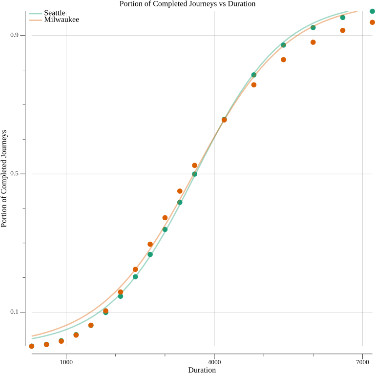
Milwaukee parameters: k=0.001049 x₀=3585
Beginning at a 70 minute time budget, Seattle’s access climbs above Milwaukee’s, and stays there as duration increases. This muddles the relationship between the presumed quality of transit in these cities. In the aforementioned comparative analysis, I suggested that King County Metro might have something to learn from Milwaukee’s transit network. With the additional information provided by the other durations, it’s now possible to question whether replicating some features of Milwaukee’s transit service could be done without having deleterious consequences. Perhaps what makes Seattle’s network worse for some durations makes it better for others. That’s not guaranteed; the superior access that Seattle sees at longer durations could be the result of geography, and not related to transit at all. There may be no danger of negatively impacting the access for large time budgets. The problem is that it’s not possible to rule this out without computing access for many durations.
The logistic functions for Milwaukee and Seattle actually predict that the access lead swaps, but the function’s poor fit undermines how significant I can find this. Milwaukee’s function performs even worse than Seattle’s at the shortest durations. The performance for the largest time budgets is worse as well. Like the comparison of the two Seattle networks, the logistic function just isn’t accurate enough to add much value.
The multi-duration comparison of Milwaukee and Seattle complicates the idea of using access to reason about the quality of transit service. It serves as a refutation of the idea that it’s sufficient to consider one time budget. Superiority at one duration does not guarantee superiority at all, or even many, of them. Adding to this complication is that a way to generalize how the access will change based on duration remains elusive.
All Models are Wrong…
“Madrona Park Loop” by Oran Viriyincy is licensed under CC BY-SA 2.0.
There’s an aphorism “all models are wrong, but some are useful”. It’s something that I take to heart in my analyses of transit. The access analyses that I produce are a model. They are a flawed and incomplete way to assess how well a public transit network will meet the needs of all individuals. Nevertheless, I believe the technique to be useful because it measures the fundamental thing that people expect from a mode of transportation: the ability to be in one place and get to another place, at a desired time, without taking too long. It’s easy to point out aspects of public transit ignored by the measurement that will impair how some person can use transit. But in the broad view, the model is measuring something aligned with the purpose of the system.
Within the overall model of access measurement, there is a compelling benefit to construct an inner model that predicts access for a duration. Computing access over multiple durations is not prohibitively expensive, but evaluating a single-variable function is extremely cheap. The comparison of Milwaukee and Seattle reveals that a city with better access at some durations isn’t guaranteed to maintain that superiority for all of them. There is a need to reasonably predict access for any time budget. The ability to derive an accurate function from a few durations would be incredibly useful. Unfortunately the logistic functions that I produced were not up to the task. They were not a useful model because they were incredibly wrong for some durations.
This doesn’t end the search for a better model. The relationship between access ratio and duration, across multiple transit networks and cities, looks too systematic to defy approximation with a closed-form expression. There are an abundance of sigmoid functions—functions that, like the logistic function, are S-shaped—that could be worth exploring.
This is all in service of making less-limited statements about transit quality. A transit planner will no longer need to fixate on crutches like Marchetti’s constant, that focus on what the average person does, because they can understand what a transit network is capable of providing at any time budget. When tradeoffs must be made, they can hew toward typical behavior, but not all changes involve tradeoffs. A model for understanding access versus duration contributes to a more aspirational approach to transit planning. It helps set individuals free from conforming to the strictures imposed by transit networks designed around averages.